Ramsauer Townsend Effect in a Xenon Thyratron

Exploring Quantum Interference: A Detailed Analysis of the Ramsauer–Townsend Experiment

In this post, I dive deep into the quantum mechanics behind the Ramsauer–Townsend effect, with a special focus on the rigorous analysis of uncertainties, results, and the derivation of the spherical 3D square well model used to estimate the potential depth of the xenon atom.

Introduction

The Ramsauer–Townsend effect is a striking demonstration of quantum mechanics where low-energy electrons scatter off noble gas atoms, such as xenon, with an anomalously low probability at specific energies. This phenomenon arises from the wave–particle duality of electrons and the resulting interference effects when electron waves traverse the potential well of an atom. In our experiment, conducted with a xenon thyratron, we observed a clear scattering minimum which, after corrections, aligned well with theoretical predictions.

Theoretical Background

Quantum Scattering and Interference

When electrons encounter a xenon atom, they experience a potential well that alters their de Broglie wavelength:

\[\lambda = \frac{h}{\sqrt{2mE}}\]

Inside the atom, the wavelength changes due to the potential, resulting in partial reflection and transmission. This change sets up conditions for destructive interference when the phase difference between the reflected waves reaches a critical value, leading to a marked minimum in the scattering cross-section.

Energy Corrections

A critical aspect of the experiment was correcting the electron energy to account for:

• Contact Potential (\(V_c\)): Due to differences in work functions between the cathode and the shield.
• Mean Emission Energy (\(V_e\)): Resulting from the thermal distribution of the emitted electrons.

The effective accelerating voltage is given by:

\[V_{\text{eff}} = V - V_s + V_c + V_e\]

Incorporating these corrections shifted the observed scattering minimum from around 0.920 eV to a corrected value of 1.006 eV, demonstrating the importance of precision calibration.

Experimental Setup and Data Collection

Apparatus Overview

The experiment used a 2D21 xenon thyratron, divided into three regions:

1. Electron Emission: A thermionically heated cathode emits electrons.
2. Scattering Region: Electrons traverse a xenon gas at approximately 0.05 Torr.
3. Detection: A plate collects transmitted electrons, while a shield grid captures the scattered ones.

For reference, see the schematic below:

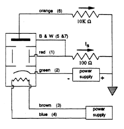
Figure 1. Schematic of the experimental setup.

Data Acquisition and Calibration

• Electron Acceleration:
  The accelerating voltage was varied between 0 and 15 V to adjust electron energies. The shield voltage was crucial in determining the effective electron energy.

• Freezing Xenon:
  Immersing the thyratron in liquid nitrogen effectively “froze out” xenon scattering, allowing for accurate calibration of the collection geometry.

• Measurement Protocol:
  Multimeters measured voltages across resistors (100 Ω and 10,000 Ω). These voltage readings were converted into currents to compute the scattering probability \(P_s\).

Detailed Uncertainty Analysis

Error Propagation

A thorough error analysis was essential for robust results. Uncertainties arose from several sources:

• Resistor Tolerances: A 5% tolerance contributed to the current measurements.
• Voltage Measurements: Finite resolution of the multimeters (e.g., ±0.0005 V for low voltages) and calibration uncertainties.
• Environmental Factors: Electronic noise and digitization errors.

The uncertainty in the current derived from a voltage measurement was propagated using:

\[\delta \left(\frac{V}{R}\right) = \sqrt{\left(\frac{\delta V}{R}\right)^2 + \left(\frac{V\, \delta R}{R^2}\right)^2}\]

This expression (Equation 24 in the lab report) was applied consistently throughout the data analysis, ensuring that uncertainties in both voltage and resistance were properly considered.

Analysis of Scattering Probability

When calculating the probability of scattering using:

\[P_s = 1 - \frac{I^*_s I_p}{I_s I^*_p}\]

the uncertainties were carefully propagated according to:

\[\delta P_s = \sqrt{\left(\frac{\partial P_s}{\partial I_p}\delta I_p\right)^2 + \left(\frac{\partial P_s}{\partial I_s}\delta I_s\right)^2 + \cdots }\]

Each partial derivative quantifies the sensitivity of \(P_s\) to the measured currents.

Statistical Fitting and Chi-Squared Analysis

To determine the minimum scattering energy precisely, a quadratic function was fitted to the data near the minimum. However, the fitting process was complicated by uncertainties in both the independent (electron momentum) and dependent (scattering probability) variables. By defining an effective uncertainty:

\[\sigma_{\text{eff}} = \sqrt{(\delta y)^2 + \left(2A(x-x_0)\delta x\right)^2}\]

we combined the x and y uncertainties before applying the fit.

Two sets of fits were performed:

• Fitting X Uncertainties Alone: Yielded a minimum at \(0.920 \pm 0.021\) eV.
• Fitting Y Uncertainties Alone: Yielded a minimum at \(0.921 \pm 0.016\) eV.

A combined fit using the scipy.odr method produced a smaller uncertainty (\(0.920 \pm 0.002\) eV), but the more conservative value of \(\pm 0.022\) eV was adopted to better reflect experimental conditions.

Chi-squared analysis further validated the fits:

• The left fit gave a reduced chi-squared near unity (1.149) with a p-value of 0.296.
• The right fit yielded a reduced chi-squared of 0.238 and a p-value close to 1, suggesting slightly overestimated uncertainties.

The final corrected scattering minimum of 1.006 ± 0.024 eV is therefore both robust and reliable.

Derivation of the Spherical 3D Square Well

A central theoretical model used in the experiment is the spherical (3D) square well, which describes the effective potential of a xenon atom. This model is key to understanding how the scattering minimum is related to the potential depth.

The Potential and Radial Schrödinger Equation

Consider a spherically symmetric potential defined as:

\[V(r) = \begin{cases} -V_0, & r < a \\ 0, & r \ge a \end{cases}\]

where \(V_0 0\) is the depth of the well and \(a\) is the effective radius of the atom.

For a particle with energy \(E\) (with \(E 0\)) incident on this potential, the radial part of the Schrödinger equation for the \(l=0\) (s-wave) is:

\(\frac{d^2u(r)}{dr^2} + k^2 u(r) = 0 \quad (r \ge a)\) \(\frac{d^2u(r)}{dr^2} + k_1^2 u(r) = 0 \quad (r < a)\)

with:

\[k = \sqrt{\frac{2mE}{\hbar^2}}, \quad k_1 = \sqrt{\frac{2m(E+V_0)}{\hbar^2}}\]

Solutions Inside and Outside the Well

The general solutions for the radial function \(u(r) = rR(r)\) are:

• For \(r < a\): \(u(r) = A \sin(k_1 r)\)
• For \(r \ge a\): \(u(r) = B \sin(kr + \delta)\)

Here, \(\delta\) is the phase shift due to the scattering potential.

Boundary Conditions and Matching

At \(r = a\), the wave function and its derivative must be continuous:

1. Continuity of \(u(r)\): \(A \sin(k_1 a) = B \sin(ka + \delta)\)
2. Continuity of the derivative \(u'(r)\): \(A k_1 \cos(k_1 a) = B k \cos(ka + \delta)\)

Dividing the derivative matching condition by the continuity condition, we eliminate the constants \(A\) and \(B\):

\[\frac{k_1 \cos(k_1 a)}{\sin(k_1 a)} = \frac{k \cos(ka + \delta)}{\sin(ka + \delta)}\]

This can be rearranged as:

\[k_1 \cot(k_1 a) = k \cot(ka + \delta)\]

For a scattering minimum (where the phase shift \(\delta \approx \pi\) or where destructive interference minimizes the scattering cross-section), this relation simplifies. Under the assumption \(ka \ll 1\) (a low-energy approximation), \(\cot(ka + \delta) \approx \cot(ka)\), and one obtains a condition that links \(V_0\) to the observed energy \(E\). Rearranging further, we arrive at:

\[E + V_0 \approx \frac{\hbar^2}{2m} \left(\frac{4.493}{a}\right)^2\]

where \(4.493\) is the first nontrivial solution to the equation \(\tan(x) = x\). This result allows us to estimate the well depth \(V_0\) given the experimental energy \(E\) at which the scattering minimum occurs.

Significance

This derivation of the spherical 3D square well model is critical because:

• It connects the experimental observable (the scattering minimum energy) to the intrinsic property of the xenon atom (the potential well depth \(V_0\)).
• It underscores the importance of quantum interference in determining the transmission properties of electrons through the atomic potential.

Detailed Results and Figures

Raw and Corrected Data

• Raw Data Analysis:
  The initial uncorrected data yielded a scattering minimum at 0.920 ± 0.022 eV.
  
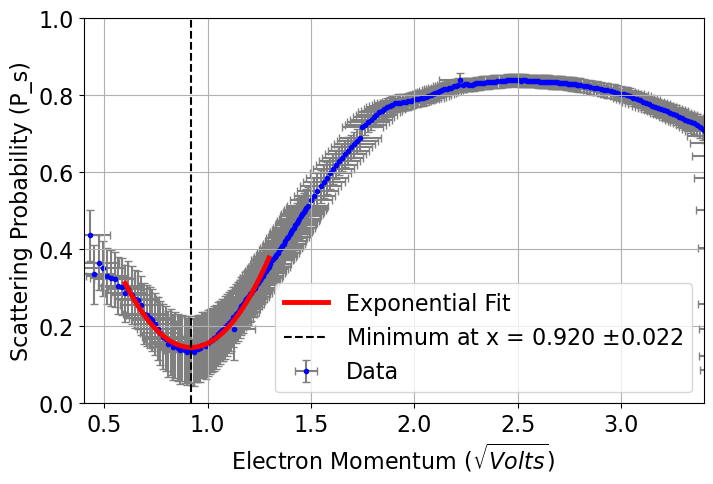
  Figure 3. Raw scattering probability as a function of \((V - V_s)^{1/2}\).

• Corrected Data Analysis:
  After applying corrections for \(V_c\) and \(V_e\), the effective electron momentum was recalculated, shifting the scattering minimum to 1.006 ± 0.024 eV.
  
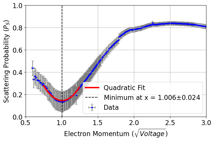
  Figure 5. Corrected scattering probability versus electron momentum.

Additional Measurements

• Reciprocal Mean Free Path:
  From \(P_s = 1 - e^{-l/\lambda}\), we calculated a reciprocal mean free path of 0.216 ± 0.0375 cm⁻¹.
  
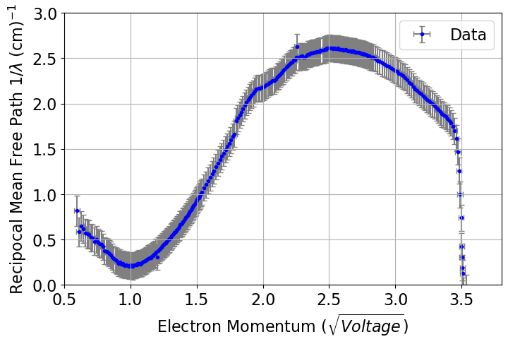
  Figure 6. Reciprocal mean free path as a function of \((V - V_s)\).

• Determination of \(V_c\) and \(V_e\):
  Linear fits of the shield current data provided values for the contact potential and mean emission energy.
  
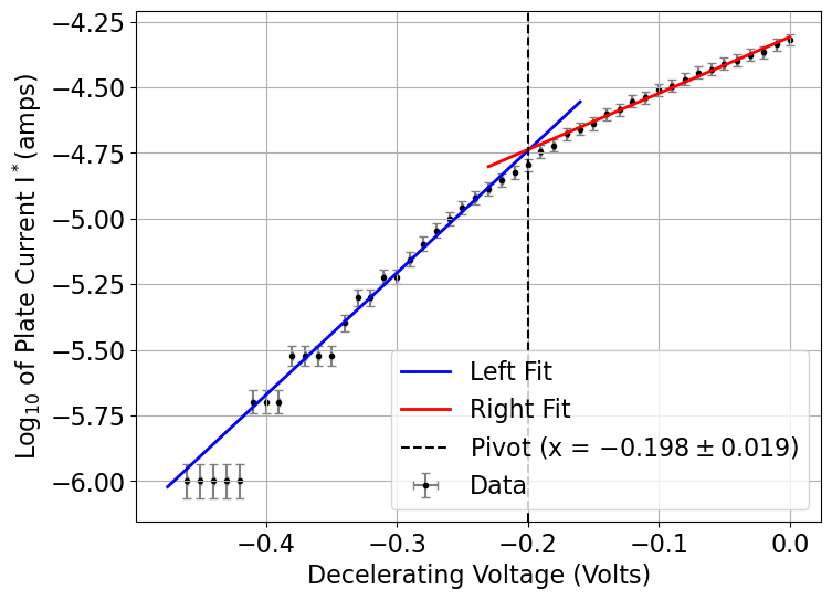
  Figure 4. Linear fit used to determine \(V_c\) and \(V_e\).

Discussion and Conclusions

The detailed analysis of uncertainties underscores the importance of rigorous error propagation in experimental physics. Our work highlights that:

• Minor Systematic Errors Matter:
  Small deviations in voltage measurements or misestimation of resistor tolerances can shift the observed scattering minimum significantly.

• Statistical Methods Enhance Reliability:
  By combining uncertainties in both variables and using chi-squared analysis, we ensured that our determination of the scattering minimum is statistically robust.

• Quantum Interference is Evident:
  The corrected minimum of 1.006 ± 0.024 eV aligns well with theoretical predictions, reinforcing the role of quantum interference in the phenomenon.

Furthermore, the derivation of the spherical 3D square well provides a solid theoretical foundation linking the observed energy minima to the intrinsic potential well depth of xenon. This comprehensive approach—from rigorous uncertainty analysis to detailed theoretical derivation—demonstrates the depth of experimental and analytical techniques required to probe quantum phenomena.

I hope this deep dive into our methodology, uncertainty analysis, and theoretical derivation inspires you to explore the precision and beauty of experimental physics further. For any questions or further discussion, feel free to reach out!

Happy experimenting!